


Key takeaways
• Match the algorithm to broken assumptions, not to a leaderboard. Anomalies are rare, mostly unlabelled, and drift over time. Pick the method that survives those three facts.
• Six families cover most real deployments. Isolation Forest, ECOD/COPOD, Local Outlier Factor, One-Class SVM, autoencoders, and a time-series model (LSTM or Anomaly Transformer). The rest are variations on these.
• The 2026 buy option shrank. Azure’s Anomaly Detector retires 1 October 2026 and Amazon Lookout for Metrics shut down in October 2025. Survivors fold detection into platforms (BigQuery ML, OpenSearch, Datadog, Elastic), which changes build-vs-buy.
• Your metric decides your fate. Accuracy and ROC-AUC lie under 0.5% anomalies. Report AUC-PR and recall-at-fixed-precision, and avoid the point-adjustment trap that lets random scores beat published state of the art.
• Most failures are operational, not algorithmic. Class imbalance, weak labels, concept drift, and alert fatigue kill more projects than model choice. Plan calibration, suppression, and a feedback loop before you pick a library.
Why Fora Soft wrote this playbook
Anomaly detection sits where three things we ship every quarter meet: real-time data pipelines, computer vision, and applied machine learning. Our AI integration team has wired ML-driven monitoring and behaviour detection into healthcare, fintech, security, and SaaS products since 2005, across 250+ delivered projects. This guide is opinionated toward the person who will own the on-call pager, not the Kaggle leaderboard.
One concrete example grounds a lot of the advice below. VALT, our HD video-evidence platform, runs across 2,500+ cameras and 50,000+ users in 770+ US organisations, including law-enforcement and medical-education customers. Detecting “something unusual” in millions of hours of stream without drowning operators in alerts is a problem we have had to solve for real, at a scale where a bad false-positive rate is a staffing budget, not a chart.
So this is the playbook we wish we had at the start: which anomaly detection algorithms actually pull their weight in production, how to choose between them, what the tooling looks like now that two of the big-cloud services have been retired, and where the build-vs-buy line really sits in 2026.
What anomaly detection actually is
An anomaly is any data point, sequence, or pattern that deviates from a system’s expected behaviour. Anomaly detection is the task of learning what “normal” looks like from observed data, usually unlabelled, then flagging what does not fit. Anomaly detection algorithms are the specific models that do the flagging.
Three shapes of anomaly dominate the field. Point anomalies are single values outside the normal range: a $50,000 charge on a card that usually buys coffee. Contextual anomalies are normal in isolation but wrong for the setting: 25°C in Stockholm in February. Collective anomalies are sequences whose individual values look fine but whose pattern does not: a server quietly serving 100 requests a minute when this hour normally sees 10,000.
The task is hard for three reasons that never go away. Anomalies are rare, often under 1% of the data. They are unlabelled or labelled inconsistently. And the definition of “normal” drifts as the world changes. Pick algorithms and an operating model that survive those three facts and most of the engineering follows.
Scoping anomaly detection for your product?
Thirty minutes with our ML lead and you leave with the right algorithm, a data-readiness checklist, and an Agent-Engineering-accelerated timeline.
Where anomaly detection algorithms pay off in 2026
The global anomaly-detection market was about $4.33B in 2022 and is projected to reach $14.59B by 2030 at a 16.5% CAGR, per Grand View Research. That spend concentrates in a handful of places where a missed anomaly is money or safety.
1. Fraud and financial crime. The single largest buyer. Every false negative is direct loss and every false positive is a furious customer, so BFSI teams invest heavily: real-time card fraud, anti-money-laundering transaction monitoring, account-takeover detection. Production stacks pair a supervised gradient-boosted head (XGBoost, LightGBM) with an unsupervised detector such as Isolation Forest or an autoencoder on transaction graphs.
2. ITOps, observability, and SRE. Where most engineers actually meet anomaly detection. Datadog Watchdog, Dynatrace Davis, Splunk ITSI, Elastic ML, Grafana ML. Time-series outliers on metrics, log anomalies, trace anomalies. Winners are cheap and boring: STL decomposition for seasonality, median-absolute-deviation for latency monitors, an Anomaly Transformer only where multivariate signals justify it.
3. Predictive maintenance and industrial IoT. Vibration, temperature, current draw, and acoustic signatures from turbines, pumps, and CNC machines. On these noisy, high-dimensional sensor streams a hybrid stack, a reconstruction model paired with a tree detector, consistently beats either model alone, which is why we default to two detectors with different inductive biases rather than chasing a single accuracy score.
4. Cybersecurity and intrusion detection. Network-flow anomalies, lateral movement, beaconing, endpoint detection. NSL-KDD and CIC-IDS-2017 remain the academic baselines; production stacks combine supervised classifiers for known tactics with unsupervised models for zero-day patterns.
5. Video and behavioural surveillance. Where we have shipped most: unusual movement, loitering, falls, perimeter breaches in CCTV. Deep models (3D CNNs, video transformers) sit behind a domain-specific suppression layer so operators are not buried. We go deeper in our reads on real-time anomaly detection in video surveillance and AI-based surveillance systems.
6. Healthcare monitoring. ECG arrhythmia detection, sepsis early warning, ICU vitals deterioration. Heavily regulated (FDA SaMD in the US, MDR in the EU), so models skew conservative and carry an explainability layer.
7. Manufacturing visual QC. Self-supervised image models such as PatchCore and PaDiM on MVTec-AD-style defect data. They reach up to 99.6% image AUROC on the clean public benchmark; expect 5–15 points lower in a real factory.
The algorithm families, organised by what you need
The literature lists dozens of named anomaly detection algorithms. In production we reach for roughly six families, chosen by data shape and how much labelled data exists. Figure 1 maps them.
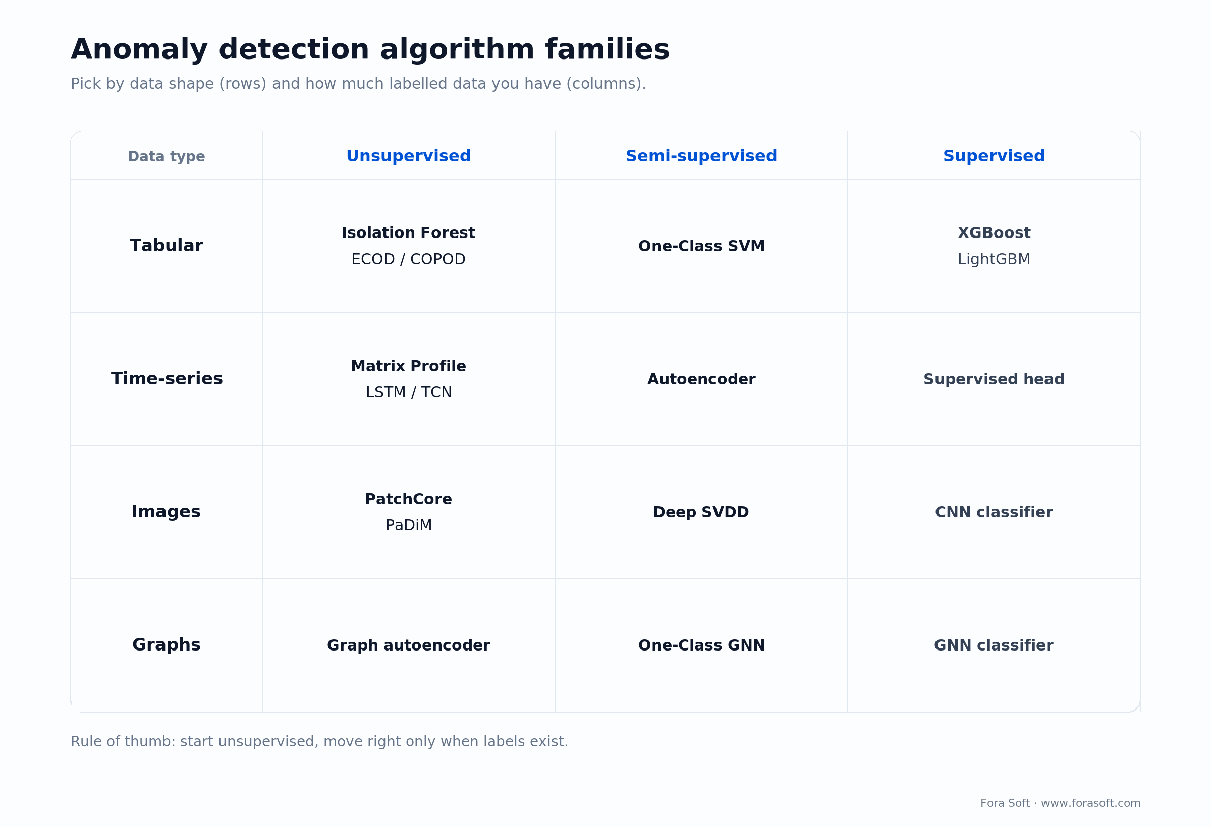
Figure 1. Anomaly detection algorithm families by data type and supervision mode — what wins on which data shape.
Isolation Forest
An ensemble of random trees that isolates points with recursive random splits. Anomalies need fewer splits to isolate, so they get shorter average path lengths. Roughly linear time, sub-sampling scales it to millions of rows, almost no tuning. Sweet spot: tabular fraud, structured logs, IoT telemetry. It is weaker on local-density anomalies, which is exactly what LOF is for.
ECOD and COPOD
Probability-based detectors that estimate the empirical CDF per feature (ECOD) or the copula structure (COPOD). Parameter-free, deterministic, explainable, and fast, they are the fastest parameter-free detectors and a strong baseline in the ADBench study of 30 algorithms over 57 datasets, where no single unsupervised method dominates. Run one as a baseline before you reach for deep learning.
Local Outlier Factor and DBSCAN/HDBSCAN
Density-based methods. LOF scores how much a point’s local density deviates from its neighbours, so it catches local outliers in variable-density data. DBSCAN and HDBSCAN cluster dense regions and label the rest as noise. Both shine when local density carries the signal, and both get slow and memory-hungry on high-dimensional or very large sets.
One-Class SVM and Deep SVDD
One-Class SVM learns a kernel boundary that encloses the normal class; useful when you have plenty of clean normal data and almost no anomalies. Training is O(n²–n³) and sensitive to the kernel and the nu parameter, so scikit-learn ships a linear-time SGD approximation for large data. Deep SVDD is the neural version: it maps normal data into a minimum-volume hypersphere in latent space.
Autoencoders and Variational Autoencoders
Train a network to reconstruct normal data; a large reconstruction error signals an anomaly. Variants run from vanilla AE to VAE, adversarial AE, and memory-augmented MemAE. Strong on high-dimensional inputs such as images, sensor arrays, and network packets, and hungrier for clean training data than the tree methods.
Time-series: LSTM, TCN, Anomaly Transformer, Matrix Profile
For sequential data with temporal dependence. LSTM and TCN forecasters score the residual between prediction and reality. Matrix Profile is a deterministic motif-and-discord detector that needs almost no tuning. The Anomaly Transformer (ICLR 2022) uses association discrepancy and is a common choice for multivariate metrics; TranAD and TimesNet are newer options worth benchmarking.
Image-specific: PatchCore, PaDiM, EfficientAD
Feature-bank methods on top of pretrained backbones. They dominate MVTec AD and fit industrial inspection, medical-imaging triage, and visual surveillance. There is a real training trade-off: PaDiM trains in about 9 seconds per category, PatchCore in about 280, in exchange for higher accuracy.
Anomaly detection algorithms compared at a glance
| Algorithm | Best for | Data shape | Strength | When it breaks |
|---|---|---|---|---|
| Isolation Forest | Fraud, logs, IoT | Tabular, mid-dim | Linear scaling, low tuning | Local-density anomalies |
| ECOD / COPOD | First baseline | Tabular, any dim | Parameter-free, explainable | Complex non-linear structure |
| LOF / HDBSCAN | Local-density anomalies | Tabular, low-mid dim | Captures clusters and noise | Large, high-dim data |
| One-Class SVM / Deep SVDD | Plentiful normal, scarce abnormal | Tabular, image features | Bounded false-positive rate | Kernel and scaling sensitivity |
| Autoencoders / VAE | High-dim, image, packets | Image, sensor, embedding | Rich non-linear normal manifold | Data-hungry, drift-sensitive |
| LSTM / TCN forecaster | Metric residuals | Time-series | Native temporal modelling | Heavy retraining on drift |
| Anomaly Transformer | Multivariate observability | Time-series | Strong on SMD/SMAP/MSL | Compute-hungry inference |
| Matrix Profile | Motif and discord | Time-series | Deterministic, no training | Best on lower-dim signals |
| PatchCore / PaDiM | Industrial visual QC | Images | Up to 99.6% AUROC on MVTec AD | Needs reference normal images |
Reach for Isolation Forest first when: your data is tabular and reasonably large. It is the most reliably good first model, and it gives you a baseline number to beat before anything fancier earns its keep.
Reach for the Anomaly Transformer when: you have multivariate time-series with real cross-channel dependencies and a GPU budget for inference. Below that bar, a forecaster plus residual scoring wins on cost.
Supervised, semi-supervised, unsupervised: how to choose
Unsupervised is the default and the most honest starting point. You have unlabelled data, mostly normal, and need to flag what does not fit. Isolation Forest, ECOD, LOF, DBSCAN, and autoencoders all live here.
Semi-supervised assumes a clean sample of normal data for training but no labelled anomalies. One-Class SVM, Deep SVDD, and autoencoders trained on normal-only data fit here. It is the common case in regulated industries where normal is curated and abnormal events are too rare to label.
Supervised is the rare luxury of both classes labelled: confirmed card-fraud chargebacks, confirmed equipment failures. Cost-sensitive XGBoost, LightGBM, and the supervised heads of multi-task networks dominate. Watch the imbalance; report PR-AUC and recall-at-fixed-precision, not ROC-AUC.
Here is the unsupervised baseline we start almost every tabular engagement with. Ten lines of scikit-learn, and you have a number to beat:
from sklearn.ensemble import IsolationForest

# X_train: mostly-normal rows; contamination = expected anomaly rate
clf = IsolationForest(n_estimators=200, contamination=0.01, random_state=42)
clf.fit(X_train)

scores = clf.decision_function(X_test)  # lower score = more anomalous
flags  = clf.predict(X_test)            # -1 = anomaly, 1 = normal
Set contamination from your real anomaly rate, not the default. Keep decision_function scores rather than the hard label so a calibration layer can turn them into a comparable percentile later. This is the whole point of a baseline: cheap, explainable, and honest about what a harder model has to beat.
Tooling in 2026: libraries, cloud, and SaaS
| Layer | Examples | When it wins |
|---|---|---|
| Library | PyOD, scikit-learn, DeepOD, Anomalib, Darts, STUMPY | Custom build, full control of the model |
| Cloud ML platform | Vertex AI, SageMaker, Databricks, BigQuery ML | You already live in that cloud and need MLOps |
| Observability SaaS | Datadog Watchdog, Dynatrace Davis, Splunk ITSI, Elastic ML | Metrics, logs, traces, no model team |
| Fraud / risk | Sift, Feedzai, NICE Actimize, Stripe Radar | BFSI buyers, regulated risk pipelines |
| Industrial / IoT | Seeq, AWS IoT SiteWise, Uptake | Manufacturing, energy, oil and gas |
| Image / video | Anomalib, custom CV pipelines | Visual QC, surveillance, medical imaging |
If you are building, start with PyOD. It ships more than 60 detectors behind one scikit-learn-style API across tabular, time-series, graph, and image data; PyOD 2 added a dozen deep models in PyTorch and an LLM-assisted model-selection workflow. Pair it with scikit-learn 1.9 for the classical estimators (IsolationForest, LocalOutlierFactor, OneClassSVM, EllipticEnvelope) and DeepOD or Anomalib when you need deep or visual detectors.
Which managed services survived 2026
This is the part most guides have not caught up with. The point-and-click, first-party anomaly APIs from the big clouds are being wound down. Microsoft’s Azure AI Anomaly Detector stopped accepting new resources in September 2023 and retires fully on 1 October 2026; Metrics Advisor, built on it, retires in the same wave. Amazon closed Lookout for Metrics to new customers in October 2024 and ended support on 10 October 2025. If your architecture diagram still has either box, it is already legacy.
The survivors did not disappear; they folded detection into a broader platform. Google’s anomaly detection lives inside BigQuery ML (ML.DETECT_ANOMALIES over ARIMA_PLUS, k-means, PCA, and autoencoders, with a newer path running on the TimesFM foundation model). Datadog Watchdog and Elastic ML still ship anomaly detection as a core feature. AWS now points Lookout users at OpenSearch, CloudWatch, Redshift ML, and QuickSight. The lesson: buy anomaly detection as a feature of a platform you already use, not as a standalone API that a vendor can sunset from under you.
Reach for a platform feature when: your anomaly detection rides on data already in Datadog, Elastic, or BigQuery. Reach for a library when the detector is a differentiated part of your product, not a monitoring afterthought.
Stranded on a retiring anomaly detection service?
We migrate teams off sunset APIs like Azure Anomaly Detector and Lookout for Metrics onto durable open-source or platform-native stacks, without losing detection quality.
Benchmark datasets that matter
Tabular and ITOps. ADBench (30 algorithms over 57 datasets) is the reference tabular benchmark; use it to justify a choice rather than trusting a single paper. NSL-KDD and CIC-IDS-2017 cover network intrusion; the Numenta Anomaly Benchmark (NAB) scores streaming time-series with an online-aware metric.
Time-series. SMD (Server Machine Dataset), NASA’s SMAP/MSL telemetry, and SWaT (industrial water treatment) are what most multivariate papers report on. Each carries known label caveats, so treat published numbers as upper bounds, not promises.
Images and video. MVTec AD is the standard industrial-defect set; BTAD and VisA extend it. For video, UCSD Pedestrian, ShanghaiTech, and UCF-Crime map to surveillance use cases like those in our video-surveillance models guide.
Metrics that survive class imbalance
Never trust accuracy here. If 0.5% of points are anomalies, a model that predicts “normal” for everything scores 99.5% accuracy and catches nothing. Worked through: on a 200,000-row stream with 1,000 true anomalies, a detector that flags 2,000 points at 40% precision catches 800 of them (recall 0.8). ROC-AUC can still read about 0.95 because the 199,000 normal points dominate the false-positive rate. AUC-PR on the same run drops toward 0.6 and tells you the truth about the alert queue.
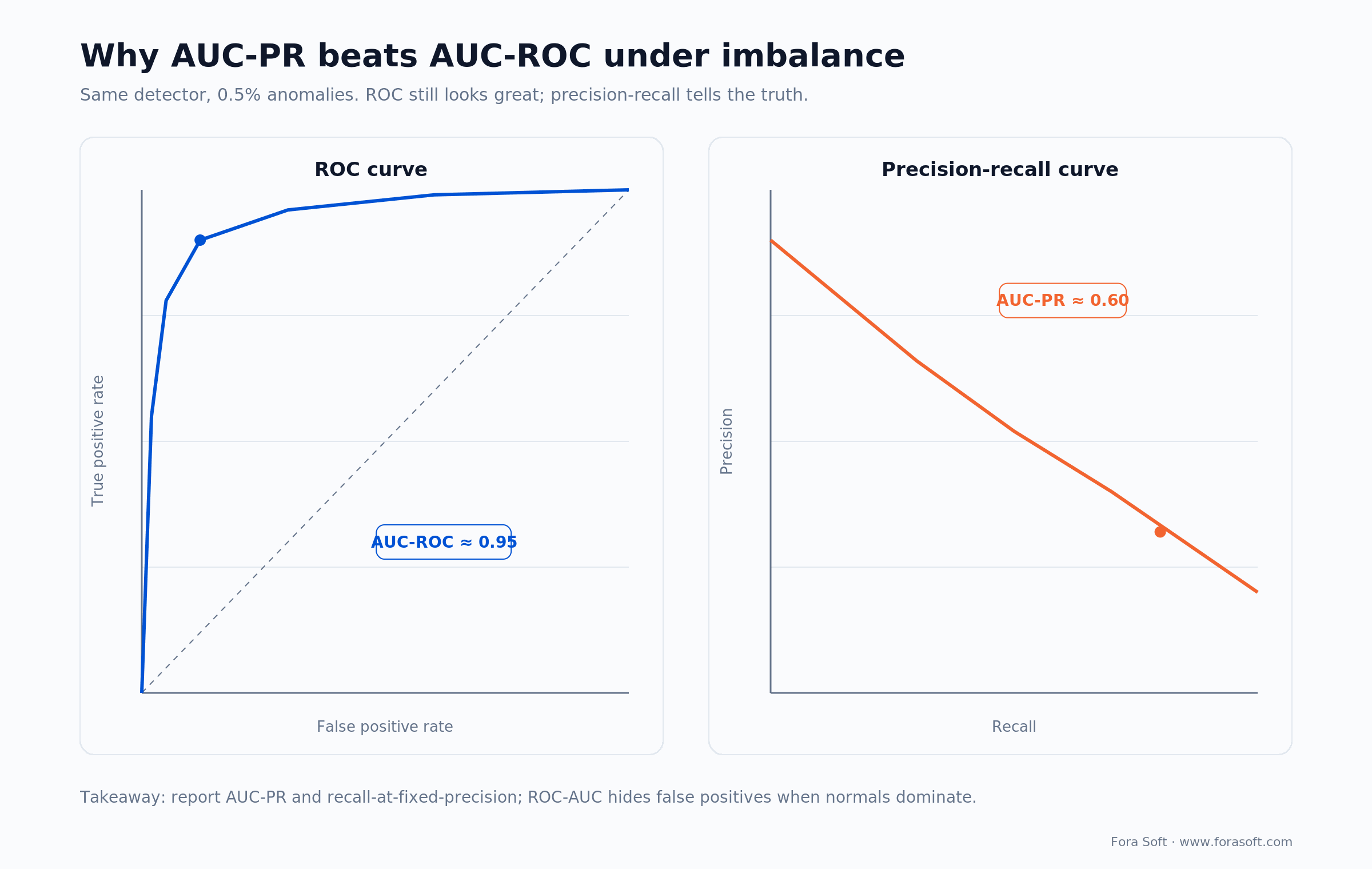
Figure 4. Under heavy imbalance, ROC stays flattering while the precision-recall curve exposes the real false-positive cost.
Use AUC-PR (average precision) as the headline, and report recall-at-fixed-precision (for example, recall at 95% precision) because that is the number product owners feel. F1@k evaluates the top-k flagged points, which mirrors an operator’s daily triage queue.
One trap that sinks time-series evaluation: point-adjustment. The popular point-adjustment protocol counts a whole true-anomaly segment as detected if the model flags even one point inside it. Kim et al. (AAAI 2022) showed that a random anomaly score can beat published state of the art under point-adjusted F1, which means a lot of “SOTA” leaderboard numbers are noise. Prefer range-based precision and recall, affiliation metrics, VUS-ROC/PR, or the PA%K variant. If a vendor quotes point-adjusted F1 with no range-based number beside it, discount it.
Reference production architecture
Figure 2 is the architecture we standardise on. It is deliberately ensemble-friendly and feedback-loop-first, because those are the two things that keep an anomaly system alive past launch.
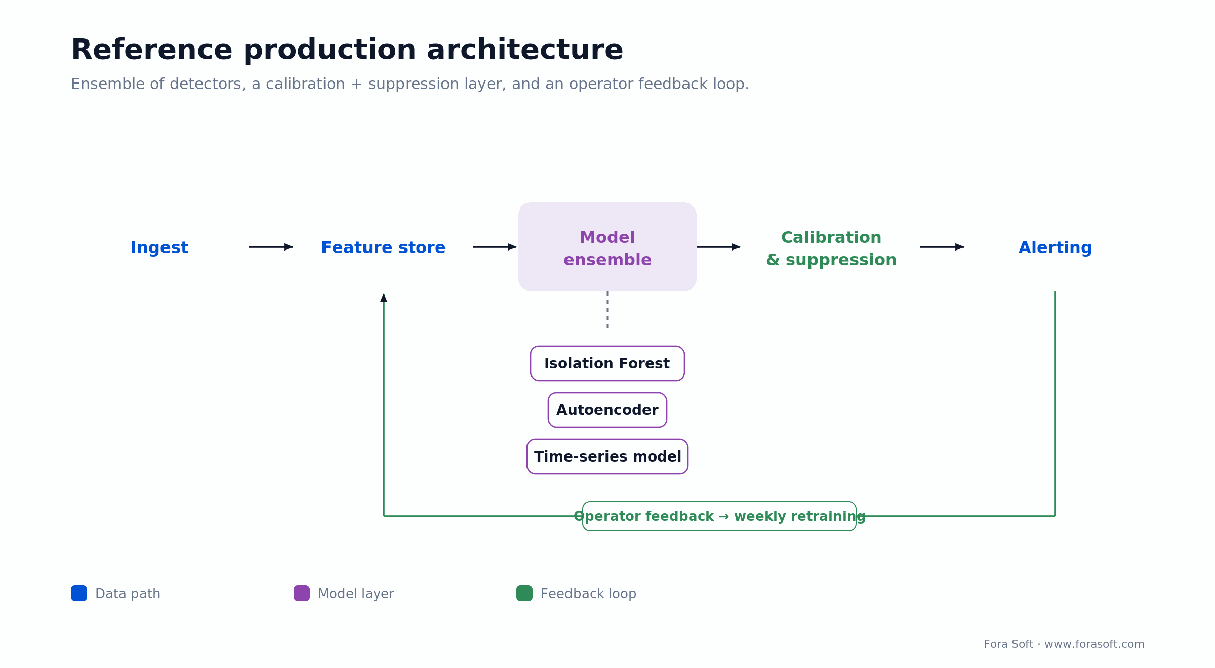
Figure 2. Reference production anomaly detection architecture used across our deployments.
Three pieces are non-obvious and carry most of the value. The calibration layer turns raw scores from very different models into a comparable percentile rank, so an Isolation Forest score and an autoencoder error can share one threshold. The suppression layer applies temporal hysteresis, deduplication, and operator-tunable thresholds; it is the line between a usable system and an alert flood. The feedback channel turns operator overrides into labelled examples, drives weekly retraining, and lets you compute real precision and recall over time.
Build vs buy: a decision matrix
| Criterion | Buy (SaaS / platform) | Build (open-source) |
|---|---|---|
| Time to first signal | Days | 8–14 weeks with Agent Engineering |
| Custom domain logic | Limited to vendor templates | Anything you can express in code |
| Data residency and compliance | Vendor regions, vendor SOC 2 | Anywhere you can run a container |
| Vendor-sunset risk | Real (see Azure, Lookout) | You own the code and the model |
| Explainability | Dashboard, limited internals | SHAP, surrogate models, audit-ready |
| Wins when | Standard observability, no in-house ML team | Differentiated data, latency or regulatory limits |
Reach for hybrid when: a SaaS gives you cheap baseline alerts on infrastructure, and you build custom detectors only on the one or two dimensions where vendor accuracy is below your bar. This is the sweet spot for most B2B SaaS and fintech teams, and it is what our custom development team builds most often.
Cost model: realistic ranges, no hype
The ranges below assume our Agent-Engineering-accelerated delivery, which is why they land below typical agency numbers. Treat them as scoping ranges, not quotes; real figures depend on data, integrations, and compliance scope. When we are unsure of a number, we do not print it.
| Scope | Typical duration | Indicative build | Ongoing run-rate |
|---|---|---|---|
| SaaS configuration and dashboards | 2–4 weeks | $15k–$40k | Vendor licence, scales with volume |
| Tabular MVP (Isolation Forest + ECOD) | 6–10 weeks | $45k–$110k | Modest CPU and alert ops |
| Multivariate time-series + autoencoder | 10–16 weeks | $90k–$220k | GPU inference and MLOps |
| Regulated / safety-critical (SaMD, fraud) | 5–9 months | $200k–$600k | Audit, revalidation, dedicated ops |
A decision framework: pick the algorithm in five questions
Figure 3 walks the same five questions as a tree. Answer them in order and the shortlist writes itself.
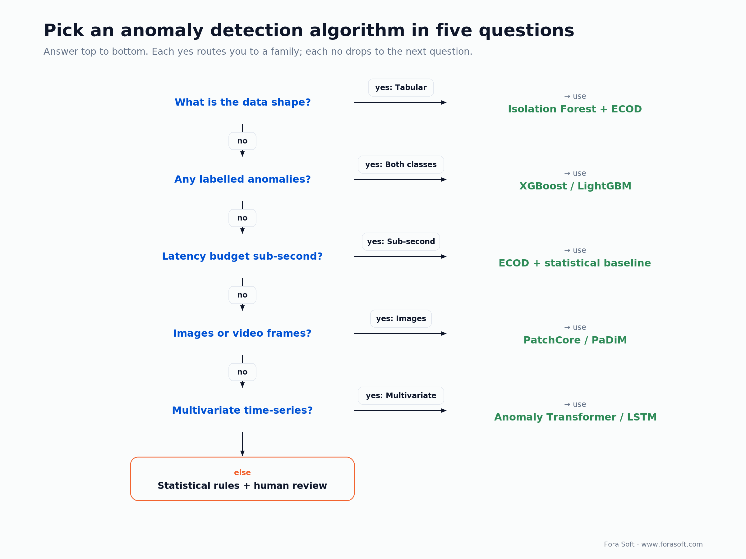
Figure 3. Pick an anomaly detection algorithm in five questions — data shape, labels, latency, actor, drift.
1. What is the data shape? Tabular points to Isolation Forest and ECOD. Time-series points to a forecaster, Matrix Profile, or the Anomaly Transformer. Images point to PatchCore and PaDiM. Graphs point to graph-native detectors. Network packets point to an autoencoder plus a supervised head.
2. How much labelled data exists? None means unsupervised. Plenty of clean normals only means semi-supervised (One-Class SVM, autoencoder on normals). Both classes labelled means supervised XGBoost or LightGBM with a cost-sensitive loss.
3. What is the latency budget? Sub-second per event favours Isolation Forest, ECOD, and lightweight statistical models. Seconds-to-minutes batch opens the door to deeper neural detectors. Hourly batch makes full ensemble retraining acceptable.
4. Who acts on the alert? An automated action with no human needs explainability, a calibrated false-positive rate, and conservative thresholds, ideally a supervised classifier in the loop. Human triage lets you run higher recall behind good suppression UX.
5. How fast does the system change? Stable distributions such as lab equipment need one training run and light refresh. Fast drift such as fraud or web traffic needs weekly or daily retraining and online algorithms like Half-Space Trees.
Pitfalls that kill anomaly detection projects
1. Optimising for ROC-AUC on a 99.5% normal class. ROC-AUC stays flattering for nonsense under heavy imbalance. Switch to PR-AUC, recall-at-fixed-precision, and F1@k from day one.
2. Ignoring concept drift. A model trained in spring will quietly degrade by autumn. Schedule weekly drift checks (population stability index, KS-test on key features) and retrain on a rolling window.
3. No feedback loop for operators. If the people who triage alerts cannot label a false positive in one click, the model never improves. Build the “mark as not anomalous” button before you build the model.
4. Shipping a single black-box model. Resilience comes from running two detectors with different inductive biases, such as Isolation Forest plus an autoencoder, and fusing them in calibration space.
5. Underspending on suppression UX. Anomaly volume is bursty. Without rate caps, deduplication, and severity tiers, operators mute the whole system inside a week and you are blind again.
KPIs: what to measure
Quality KPIs. Precision@k (target ≥ 0.7 for the top-50 daily flags), recall on a held-out labelled set (≥ 0.6 for unsupervised, ≥ 0.85 for supervised), and drift alarms per week held low and stable.
Business KPIs. Mean time to detect, mean time to resolve, prevented loss in dollars (fraud blocked, downtime avoided), and operator alert load per shift. These are the numbers a CFO signs off on.
Reliability KPIs. P95 inference latency (target under 1s streaming, under 500ms transactional), retraining cadence versus drift signal, model-version rollback time, and the share of alerts that carry an explainability output.
Mini case: detection across 2,500+ surveillance streams
Situation. Our VALT platform serves 770+ US organisations, from law enforcement to hospitals to universities, with 2,500+ HD cameras and 50,000+ users. Operators were reviewing endless footage for unusual activity, and alert fatigue was the real constraint, not model accuracy.
Approach. A hybrid stack: a cheap background-modelling detector for the first pass, a 3D CNN scene classifier for human-activity tagging, and a self-supervised reconstruction model trained on each camera’s own baseline. On top sat calibrated severity tiers, deduplication across overlapping camera fields, and per-site suppression rules tuned with the customer.
Outcome. Operators triage a fraction of the original alert volume, detection coverage extends across all 2,500+ active streams without proportional headcount, and the platform underwrites encrypted evidence chains for downstream legal use. Different vertical, same playbook every time: hybrid detectors, calibrated scores, suppression UX, feedback loop. Want a similar assessment of your stack? Book a 30-minute call and we will map it with you.
When NOT to use ML anomaly detection
Skip machine learning when a static rule already gives you 95% of the value. There is no shame in “if amount is over the threshold, hold the transaction.” Skip it when you genuinely have no historical data and no path to gather it within 6–12 months. Skip it when a false positive is catastrophic and unrecoverable, such as an autonomous medical intervention. And skip it when the team that owns the system cannot maintain a retraining pipeline, because an unmaintained model quietly rots.
The honest answer is often a blend: statistical thresholds for the obvious cases, ML for the rest, and a human reviewing the top ten flags daily. That ships in weeks, not quarters, and it is usually the right first version.
Drowning in false positives?
We have rescued anomaly detection rollouts in fintech, healthcare, and surveillance with calibration, suppression, and active-learning fixes. Bring us the noisy dashboard.
FAQ
Which anomaly detection algorithm is best?
There is no single best. For tabular data, start with Isolation Forest and ECOD as baselines. For time-series, use an LSTM forecaster or the Anomaly Transformer. For images, use PatchCore or PaDiM. The strongest production stacks combine two detectors with different inductive biases behind a calibration layer.
What are the main types of anomaly detection algorithms?
By technique: statistical (z-score, STL), distance and density (kNN, LOF, DBSCAN), tree ensembles (Isolation Forest), probabilistic (ECOD, COPOD), boundary methods (One-Class SVM, Deep SVDD), and reconstruction methods (autoencoders, VAE). By supervision: unsupervised, semi-supervised, and supervised. Match the technique to your data shape and how much labelled data you have.
Supervised or unsupervised, which should I pick?
Default to unsupervised, because anomalies are usually rare and unlabelled. Use semi-supervised when you have a clean sample of normal data. Move to supervised only when you have hundreds to thousands of labelled anomalies of a consistent type, and then use cost-sensitive XGBoost or LightGBM and report PR-AUC, not ROC-AUC.
Should I build with PyOD or buy Datadog or Splunk?
If you want anomaly detection over an existing observability stack and have no ML team, buy. If you have proprietary data, custom domain logic, or compliance needs an off-the-shelf vendor cannot meet, build with PyOD or scikit-learn. Many teams end up with both: SaaS for infrastructure metrics, custom code for the differentiated product surface.
Is Azure Anomaly Detector still available?
No new resources since September 2023, and the service retires fully on 1 October 2026, along with Metrics Advisor. Amazon Lookout for Metrics also ended support in October 2025. Microsoft points users to the open-source anomaly-detector project and Microsoft Fabric; AWS points to OpenSearch, CloudWatch, and Redshift ML. If you are starting fresh, prefer an open-source library or a platform-native feature like BigQuery ML or Datadog.
Why not just use accuracy or ROC-AUC?
Both are inflated by the huge normal class. Under 0.5% anomalies, a “predict normal” model scores 99.5% accuracy, and ROC-AUC stays high because true negatives dominate. Report AUC-PR and recall-at-fixed-precision, and for time-series avoid point-adjusted F1, which a random score can beat.
How do I keep the model from drifting?
Run weekly drift checks (population stability index, KS-test on key features), retrain on a rolling window, and feed operator feedback into the labelled set. Online algorithms such as Half-Space Trees or online Isolation Forest variants help when distributions move continuously.
Can anomaly detection run on the edge?
Yes. Isolation Forest, ECOD, and lightweight autoencoders run comfortably on edge devices via ONNX, TFLite, or Core ML. That suits IoT, on-camera surveillance, and privacy-sensitive deployments where raw data should not leave the device.
What to Read Next
Surveillance
Real-Time Anomaly Detection in Video Surveillance
Streaming detector patterns and how to keep operator alert load sane.
AI surveillance
AI-Based Anomaly Detection Surveillance System
Architectures, models, and lessons from systems we have shipped at scale.
Models
Anomaly Detection Models for Video Surveillance
A side-by-side on the deep models that hold up under live conditions.
Monitoring
Machine Learning for Real-Time Monitoring
How to wire an ML monitoring loop end-to-end without alert fatigue.
Learn
AI Security Cameras and Video Analytics Playbook
The engineering playbook for intelligent video analytics on the edge.
Ready to ship anomaly detection that moves the metric?
The right anomaly detection algorithm depends on your data shape, the labels you can produce, and how fast the world changes. Start with Isolation Forest and ECOD as a free baseline. Layer an autoencoder or Anomaly Transformer where the signal earns it. Then invest at least as much in calibration, suppression UX, and the feedback loop as in the model itself, and pick your metric before you pick your library.
One more thing worth stealing from 2026: buy detection as a feature of a platform you already run, not a standalone API a vendor can retire. We have been building ML detection into surveillance, healthcare, and SaaS products long enough to know where the cliffs are, and Agent Engineering is what lets us deliver in months instead of quarters. If you want a second opinion on the algorithm, the architecture, or the budget, we are one call away.
Get a second opinion on your anomaly detection plan
Thirty minutes with our ML lead, a clear scope and cost range, and honest advice on build versus buy.

