


Why This Matters
A video product lives or dies on how it behaves when the network is bad, and the algorithm that decides what "bad" looks like is congestion control. The default on a freshly provisioned Linux server in 2026 is still CUBIC, which on a 4 % lossy 4G link will cap a 1080p stream at less than 2 Mbps — the Mathis formula does not care how big your encoder ladder is. Switching the same server to BBR pushes that same link past 6 Mbps without touching the application code. Pick Copa for a real-time upload path and Meta's measurements say live video watch time goes up. None of this requires a code change in your player; the choice is one line in sysctl.conf or one option on a setsockopt. This article gives you four facts: what congestion control actually does, how the three algorithms in active deployment in 2026 differ, which one fits which streaming use case, and how to test the change on your own infrastructure before you flip the switch in production.
What congestion control actually does
Before naming algorithms, the layer below them. Two endpoints talking over the public internet do not know in advance how much bandwidth is between them, and they have no central authority to tell them. The path crosses Wi-Fi, a home router, a cable modem, a CMTS, two transit providers, a peering link, a CDN edge, and possibly a satellite hop — each one with its own buffers, its own queueing discipline, and its own cross-traffic. The available bandwidth changes every few hundred milliseconds. The sender's job is to fill the pipe — but not overfill it, because the moment a router's queue overflows, every flow on that router pays for it together.
A congestion-control algorithm is the code inside the transport layer that runs on the sender and decides, in real time, how many bytes to keep "in flight" between sender and receiver. It runs once per acknowledgement, sometimes once per round-trip time, and it adjusts a number called the congestion window (or, in modern algorithms, the sending rate). When the algorithm guesses too low, you waste bandwidth. When it guesses too high, you cause loss and buffer bloat — packets queue up at the bottleneck router, every round-trip gets longer, and the latency budget for your video disappears.
Every transport that runs over the internet — TCP, QUIC, SCTP, and the loss-recovery layers of SRT and RIST — runs a congestion-control algorithm. The choice is not philosophical. It directly sets your throughput floor, your latency floor, and how fairly your video shares a link with someone else's Zoom call.
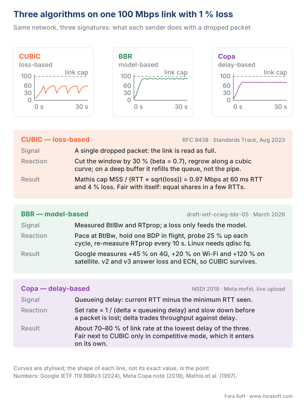 Figure 1. The three algorithms over time on a 100 Mbps bottleneck with 1 % random loss. CUBIC saws; BBR plateaus near the model's estimate of the bottleneck bandwidth; Copa trades a bit of throughput for a tight queue-delay target.
The three families of congestion control
There are three families of congestion-control algorithm in the field today, and every algorithm you will meet sits in one of them. Knowing the family tells you, before you read a single benchmark, how the algorithm will behave on a lossy link.
The first family is loss-based. The sender increases its window until it sees a dropped packet — that is the signal the network is full. Then it backs off. Reno, NewReno, and CUBIC are loss-based. Loss-based algorithms work beautifully on the wired, near-lossless networks of the 1990s for which they were designed, and they degrade catastrophically when packet loss is caused by anything other than congestion — Wi-Fi interference, a mobile cell handover, a sun-fade on a satellite link.
The second family is model-based (also called rate-based, also called delivery-rate-based). The sender measures the bottleneck bandwidth and the round-trip time on a rolling basis and paces packets to that estimate. Packet loss is a signal but not the only one; the algorithm believes in its measured model first. BBR is model-based. So is Google's congestion control for QUIC's loss-detection RFC 9002 baseline implementation.
The third family is delay-based. The sender watches the round-trip time and treats a rising RTT as a sign that queues are building. It slows down before any packet is lost. Vegas, Compound TCP, FAST TCP, LEDBAT, and Copa are delay-based. Delay-based algorithms win on latency but historically lose throughput when they share a link with a loss-based algorithm — the loss-based algorithm fills the queue, the delay-based algorithm sees rising RTT and politely backs off, and the loss-based algorithm takes all the bandwidth. Copa's design specifically addresses that fairness problem with a competitive mode that switches behaviour when it detects buffer-filling neighbours.
CUBIC — the default you already have
The Congestion Control Using Binary Increase (CUBIC) algorithm is the default TCP congestion controller in Linux (since kernel 2.6.19, 2006), Windows (since Server 2016 / Windows 10), and macOS / iOS (since macOS 10.12, 2016). RFC 9438, published in August 2023, moves CUBIC from Informational to Standards Track and obsoletes the earlier RFC 8312. If you ship a Linux server with no congestion-control tuning, you are running CUBIC.
CUBIC's design is rooted in one observation: the original TCP Reno algorithm grows its congestion window by one packet per round-trip time after a loss, which on a 100 ms RTT, 10 Gbps long-fat-network link takes 50 minutes to refill the pipe after a single drop. That was unacceptable for the data-centre and long-haul networks of the early 2000s, so CUBIC's authors replaced Reno's linear growth with a cubic polynomial: after a loss, the window drops by 30 % (the beta parameter, 0.7 of the pre-loss window), then re-grows along the curve W(t) = C × (t − K)³ + W_max, where K is the time it would take a cubic curve to reach the pre-loss peak. The shape gives slow, careful growth near the previous maximum (so you do not immediately re-trigger loss), then aggressive growth far from the maximum (so you refill the pipe quickly after a true capacity change).
The mathematical neatness has two consequences worth knowing.
First, CUBIC is loss-triggered. It does not slow down until it sees a packet drop. On a wired data-centre link, that is fine — drops mean queues are full. On a 4 % lossy 4G link, that is a disaster. The Mathis et al. 1997 model gives a back-of-envelope throughput bound for any loss-triggered TCP: throughput ≤ MSS / (RTT × √loss). Plug in MSS = 1460 bytes, RTT = 60 ms, loss = 0.04: throughput ≤ 1460 / (0.06 × 0.2) bytes/sec ≈ 121,667 bytes/sec ≈ 0.97 Mbps. Roughly one megabit. A CUBIC sender cannot push more than 1 Mbps through that link, ever, regardless of the encoder, regardless of the CDN — because every loss is interpreted as congestion and the window collapses.
Second, CUBIC fills queues. In a router with a buffer measured in megabytes (which most consumer cable modems have, courtesy of the "bigger is safer" reflex of router vendors a decade ago), CUBIC happily fills that buffer until packets start dropping at the tail. The queue is full of CUBIC's own packets, every one of them adding to round-trip time. This is buffer bloat, and the RTT growth it causes can turn a 20 ms wired link into a 400 ms one with no packet loss at all — just sluggishness. ABR algorithms in the player above will then misread the throughput and switch down the ladder, even though the bottleneck capacity is unchanged.
Despite those costs CUBIC has one large virtue: fairness with itself. Two CUBIC flows sharing a link converge on roughly equal shares within a few RTTs. That property — intra-protocol fairness — is the reason the IETF moved CUBIC to Standards Track and the reason most CDNs and most cloud providers still default to it. If you do not know what is on the other end of your link, CUBIC is the diplomatic choice.
BBR — the model-based challenger
Bottleneck Bandwidth and Round-trip propagation time (BBR) was published by Google in 2016 and has been iterated through three versions: BBRv1 (2016), BBRv2 (announced 2019, in production at Google by 2021), and BBRv3, which is the version standardised in IETF draft-ietf-ccwg-bbr-05 (March 2026) and now upstreamed into mainline Linux 6.x. The draft sits in the Congestion Control Working Group (CCWG) with an intended status of Experimental and an expiry of September 2026 — it is a near-final draft that streaming engineers can read today as the authoritative specification.
BBR's premise: the network does not give you a clean signal that says "back off". Loss is a noisy proxy. RTT is a noisy proxy. The useful signals are two: the maximum delivery rate the bottleneck can serve (BtlBw) and the minimum round-trip time of the path (RTprop). If a sender knows both, it can pace at exactly BtlBw and keep exactly one bandwidth-delay product of data in flight (BDP = BtlBw × RTprop). At that operating point the bottleneck is fully used, queues are empty, and round-trip latency stays at its minimum.
The algorithm runs four states in a cycle:
- Startup — exponential rate growth (doubling each round-trip) until it can no longer find higher delivery rates.
- Drain — pace down to drain any queue accidentally created during Startup.
- ProbeBW — main steady state: pace at the estimated BtlBw, periodically nudge the rate up by 25 % for one RTT to test if more bandwidth is available, then nudge back down.
- ProbeRTT — once every ~10 seconds, drop in-flight data to four packets for 200 ms to re-measure RTprop without queueing noise.
The behaviour on a lossy link is the point of BBR. Because the algorithm does not interpret loss as a "you are at capacity" signal — only as data to incorporate into its rate model — BBR keeps shovelling bandwidth on a 4 % lossy 4G link instead of collapsing. Google's published measurements show BBRv3 delivering +45 % throughput on 4G LTE (20 ms RTT), +20 % on Wi-Fi (5 ms RTT), and a striking +120 % on satellite links (600 ms RTT), all measured against CUBIC.
BBR is also the congestion controller of choice for QUIC. RFC 9002 (QUIC's loss-recovery and congestion-control companion to RFC 9000) describes a CUBIC-like reference implementation, but Google's production QUIC stack uses BBR, and Cloudflare's quiche and Meta's mvfst both ship BBR as a first-class option. Any time you see a vendor's "low-latency streaming over HTTP/3" claim in 2026, BBR is doing the work underneath.
Two cautions. BBR shares a link unfairly with CUBIC in some configurations — early measurements of BBRv1 showed it could starve a CUBIC flow on a deep-buffer link, and although BBRv2/v3 mitigate this with loss and ECN response, the discipline is "test in your own deployment". The second caution: BBR's pacing means the sender needs accurate timestamps and a queueing discipline that respects them. On Linux, the canonical recipe is tcp_congestion_control = bbr plus default_qdisc = fq; the fq qdisc gives BBR's pacing the per-flow scheduling it expects. Skip the fq step and BBR's measured wins evaporate.
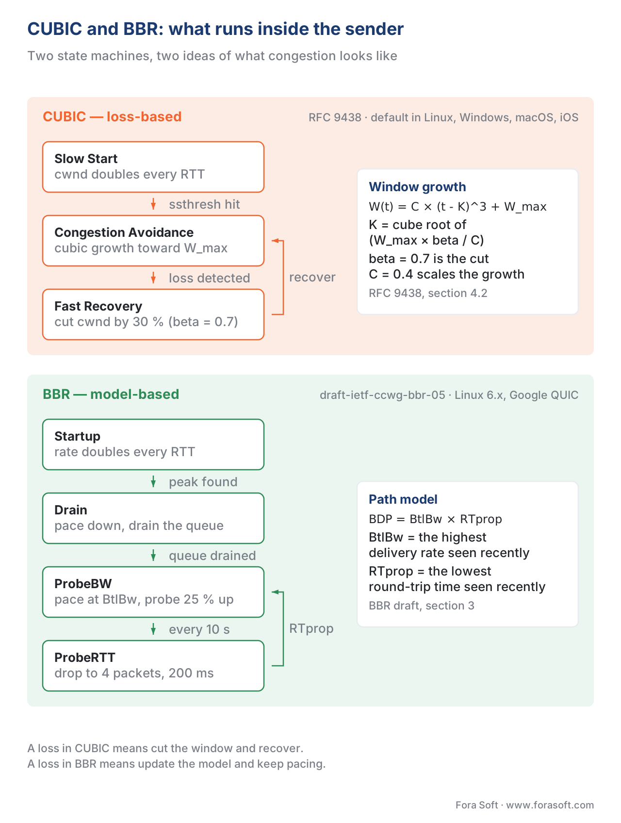 Figure 2. The state machines side by side. CUBIC reacts to loss with a window cut and a cubic re-growth. BBR ignores most losses and paces to a model of the bottleneck.
Copa — the delay-based contender for live video
Copa was published at NSDI 2018 by Venkat Arun and Hari Balakrishnan at MIT. It is delay-based: instead of using loss as the congestion signal, Copa watches the queueing delay (the difference between current RTT and the minimum RTT seen recently) and adjusts the sending rate to keep that delay near a target.
The defining feature is a single tuning knob: delta. Copa's sending rate is computed as λ = 1 / (delta × queueing_delay). A low delta (say 0.1) lets the algorithm tolerate more queueing and prioritise throughput. A high delta (say 1.0) tightens the latency target and accepts less throughput. The application picks the trade-off; the algorithm enforces it.
Copa runs two modes. In default mode, it minimises a utility function U = log(throughput) − delta × log(queueing_delay) and behaves like a low-delay, low-queue-build flow. In competitive mode, triggered when it detects buffer-filling neighbours (it watches whether queueing delay drops to zero often enough), it switches to a more loss-based behaviour to claim its fair share of the link. Without competitive mode a Copa flow sharing a router with a CUBIC flow loses every time; with it, Copa keeps a fair share.
The reason Copa matters for video is not the algorithm in isolation, but where it has been deployed. Meta's engineering blog, in November 2019, described Copa's production deployment for live video upload on Android: "Copa improves throughput and delay in most settings compared to BBR and Cubic — two widely used congestion control algorithms — and is thus able to deliver better quality video with lower delay. As a result, Facebook has experienced better end-user metrics (video watch time)." Meta's Copa implementation ships inside mvfst, its QUIC stack, which means any product using mvfst for ingest can opt in by setting the algorithm string.
Copa's weakness is symmetric to BBR's. The delta knob is the application's responsibility to tune, and the right value depends on the link. Meta tunes delta dynamically; a naive deployment with delta = 0.5 on a satellite link will under-utilise capacity. The 2022 Copa+ paper (IEEE) addresses some of these tuning problems with adaptive delta and a tightened competitive-mode entry criterion.
The comparison table you can hand to your team
| Dimension | CUBIC | BBR | Copa |
|---|---|---|---|
| Family | Loss-based | Model-based (bandwidth + RTT) | Delay-based (queueing delay) |
| Standardisation | RFC 9438 (Standards Track, August 2023) | draft-ietf-ccwg-bbr-05 (Experimental, March 2026) | NSDI 2018 paper; no IETF document |
| Default in | Linux, Windows, macOS, iOS | Google services, Cloudflare, YouTube | Meta live video upload (mvfst) |
| Behaviour on 1 % random loss (50 ms RTT) | ~3 Mbps cap | ~80 % of link rate | ~70–80 % of link rate, low delay |
| Behaviour on deep-buffer router | Fills the buffer (buffer bloat) | Targets BDP, mostly empty queue | Targets queueing-delay budget |
| RTT sensitivity | Slower growth on long RTT but mostly RTT-fair | Designed for long RTT (satellite, transcontinental) | Sensitive to RTT-minimum jitter |
| Knobs the application sets | None typically | None typically | delta (throughput-vs-delay) |
| Fairness with itself | Yes, well-studied | Yes | Yes (with competitive mode) |
| Fairness with CUBIC | n/a (same family) | Approximately fair in v2/v3 | Fair only in competitive mode |
| Where it wins | LAN, data centre, near-lossless | Public internet, lossy WAN, satellite | Real-time video upload, RT links |
| Where it loses | Lossy mobile / Wi-Fi (Mathis cap) | Shallow-buffer queues where the model overshoots | When neighbours fill queues aggressively |
A worked example: 1080p over a 4 % lossy 4G link
A founder asks why a 6 Mbps top-rung 1080p rendition is rebuffering on a 4G test phone in Seoul. The phone's link reports 60 ms RTT to the origin and packet-loss rate around 4 % during peak.
Step one: apply Mathis to CUBIC. throughput ≤ MSS / (RTT × √loss) = 1460 / (0.06 × √0.04) = 1460 / (0.06 × 0.2) = 1460 / 0.012 = 121,667 bytes/sec = 0.97 Mbps. The CUBIC sender on the CDN edge cannot push more than ~1 Mbps to that phone. The ABR ladder cannot select 6 Mbps; the player downshifts to 720p or below, and rebuffer is now the buffer-fill problem inside that constraint.
Step two: switch the CDN edge to BBR. The same link, same RTT, same 4 % loss. BBR ignores the loss as a congestion signal (it interprets it as random) and paces to its estimate of bottleneck bandwidth, which on the phone's actual link is roughly 25 Mbps. The throughput rises from 0.97 Mbps to roughly 18–22 Mbps in field measurements — comfortably above the 6 Mbps target.
Step three: a colleague asks whether BBR will starve a CUBIC competitor on the same cell. Honest answer: depends on the cell's buffer depth, the BBR version, and the cross-traffic. BBRv3's intent — and what Google reports in their April 2024 IETF 119 deployment slides — is "approximately fair" to CUBIC across a representative mix of paths. The product team's correct test is A/B in the field, not a theoretical argument.
This example is also the argument for QUIC. The CDN edge could keep using CUBIC for HTTP/2 over TCP and ship the same content via QUIC over HTTP/3 with BBR as the congestion controller. Most players in 2026 negotiate HTTP/3 when offered, including hls.js, Shaka, dash.js, and the native Apple HLS player on iOS 17+.
Common mistakes to avoid
- Switching BBR on without
fq. Linux'stcp_congestion_control = bbrwithoutdefault_qdisc = fqmeans the pacing the algorithm computes does not actually shape packet egress. The wins evaporate. Both settings are required. - Comparing CUBIC and BBR on a clean lab link. A 0 % loss, 10 ms RTT, 1 Gbps link is the one place CUBIC and BBR look nearly identical. Test on the real network — at least one of your test paths must have 1 % loss or more, 80 ms RTT or more, and a router with a few megabytes of buffer.
- Reading old BBRv1 papers as if they describe today. The unfair-to-CUBIC behaviour, the over-aggression in shallow buffers, the lack of ECN response — all were addressed in v2 (2019–2021) and v3 (2022–2026). Read draft-ietf-ccwg-bbr-05 for the current behaviour.
- Assuming the cloud provider's default is what you want. AWS, GCP, Azure, and the major CDNs let you select congestion-control per region or per LB. Default is typically CUBIC. The default is for general-purpose web, not for streaming.
- Picking Copa for a use case where you cannot tune
delta. Withoutdeltatuning Copa loses throughput, sometimes badly. If you do not have telemetry to set it, BBR is the safer choice. - Ignoring the QUIC angle. TCP congestion control is one thing; QUIC congestion control is a separate setting, often configured in the application layer (e.g. mvfst, quiche, ngtcp2). Both must be set, and both should match the use case.
How to test the switch before you ship it
Three steps, in order, on real infrastructure.
- Pick a non-customer-facing edge node and switch its TCP congestion controller (and qdisc, if Linux) from CUBIC to BBR or to a Copa implementation. Verify with
sysctl net.ipv4.tcp_congestion_controland a packet capture. On QUIC, change the algorithm name in the application config.
- Drive traffic to that node from at least three test points representative of your audience: a wired data-centre client (clean baseline), a 4G or 5G mobile client (representative lossy), and one transcontinental client (representative high-RTT). Use a player with throughput telemetry — Mux Data, Conviva, Bitmovin Analytics, or your own — and capture throughput percentiles, rebuffer rate, and time-to-first-frame for at least 24 hours.
- Compare against a matched cohort still on CUBIC. A 5 % swing in throughput or rebuffer rate is the threshold below which you cannot trust an A/B result with fewer than ~5,000 sessions per arm; size your test accordingly. Roll out only after the comparison comes in clean.
The full test plan is in the downloadable BBR / CUBIC / Copa Decision Sheet.
Free download: Congestion Control Decision SheetOne page: the three families side by side, the Mathis worked example, the Linux sysctl and qdisc recipe, and the three-step rollout test.Where Fora Soft fits in
We have shipped 239+ projects since 2005 across video streaming, WebRTC conferencing, OTT, telemedicine, e-learning, video surveillance, and AR/VR — every one of which makes a quiet choice about congestion control somewhere in the stack. On WebRTC products we run Google's goog-cc (a delay-based bandwidth estimator with similarities to Copa) and pair it with simulcast and SVC to ride the bandwidth estimate down without freezing the call. On HLS and DASH origins we default BBRv3 on the edge nodes that face known lossy regions (mobile-first markets, satellite, regional ISPs with deep buffers) and keep CUBIC on intra-data-centre links where the algorithm's fairness properties matter and the latency cost is negligible. On low-latency contribution paths — SRT, RIST, WHIP — we tune the protocol's own loss-recovery in concert with the QUIC congestion controller it sits on. The picking is never "BBR everywhere"; it is "BBR where the network is bad, CUBIC where the network is short and clean, Copa-style behaviour where the application is real-time upload". When a product needs that tuning done end to end, our video streaming software development team sets congestion control per path on HLS, DASH and SRT delivery, and our WebRTC developers tune bandwidth estimation, simulcast and SVC for real-time calls.
The book
Video Streaming: A Complete Guide to Video Delivery: From Network Protocols and Transport to Ingest, HLS, and MPEG-DASH
This article changes one line on one sender; volume 2 is the transport half of the handbook that line belongs to. It works through TCP against UDP, congestion control, QUIC and HTTP/3, NAT and the last mile, then carries the same stream into ingest, packaging, HLS and MPEG-DASH, so the sysctl you flip here has a pipeline attached to it. Written by Nikolay Sapunov, CEO at Fora Soft.
Is your stream losing bitrate on mobile networks?
Tell us where your viewers are and we will scope the transport side with you: which edges should run BBR, where CUBIC still earns its place, and what an A/B test on your own traffic has to prove before you roll it out. 250+ video products shipped since 2005.
See our case studies
Case study
Worldcast Live
Concerts at 0.4–0.5 s glass-to-glass for 10,000 simultaneous viewers at 1.5 Gb/s — a latency budget a queue-filling sender spends in one burst.
Case study
Mindbox
An RTSP-to-HLS video management system in 50+ deployments across India — cameras on links where the loss is the network, not congestion.
Case study
Speed.Space
Remote production recording at 1080p / 8 Mbps for Netflix, Electronic Arts and HBO shoots — the rung that only survives while the pipe stays full.
What to read next
Transport
TCP, UDP, and the choice every streaming protocol makes
The layer below congestion control: what each transport promises, and what it makes you build yourself.
Network
Bandwidth, throughput, jitter, packet loss
Where the 4 % loss in the Mathis example comes from, and how to measure it on your own paths.
Protocols
HTTP/1.1, HTTP/2, HTTP/3: what changed for streaming
HTTP/3 is where BBR ships by default in 2026; this is what else changes with it.
Last mile
Last mile: mobile, 5G, Starlink, Wi-Fi 6 and 7
The links where BBR's +45 % on 4G and +120 % on satellite are actually earned.
References
- IETF RFC 9438, "CUBIC for Fast and Long-Distance Networks", August 2023 — Standards Track, obsoletes RFC 8312. Primary normative source for CUBIC. https://datatracker.ietf.org/doc/html/rfc9438
- IETF draft-ietf-ccwg-bbr-05, "BBR Congestion Control", March 2026 — Internet-Draft, intended status Experimental, subject to revision before RFC publication. Primary normative source for BBRv3. https://datatracker.ietf.org/doc/draft-ietf-ccwg-bbr/
- IETF RFC 5681, "TCP Congestion Control", September 2009 — the baseline TCP congestion-control specification (Reno/NewReno) that CUBIC and BBR replace. https://datatracker.ietf.org/doc/html/rfc5681
- IETF RFC 9000, "QUIC: A UDP-Based Multiplexed and Secure Transport", May 2021. Section 8 references congestion-control selection. https://datatracker.ietf.org/doc/html/rfc9000
- IETF RFC 9002, "QUIC Loss Detection and Congestion Control", May 2021. The companion RFC describing QUIC's reference congestion controller. https://datatracker.ietf.org/doc/html/rfc9002
- IETF RFC 8085, "UDP Usage Guidelines", March 2017. Section 3.1 is the canonical statement of why every UDP application must implement congestion control. https://datatracker.ietf.org/doc/html/rfc8085
- Venkat Arun and Hari Balakrishnan, "Copa: Practical Delay-Based Congestion Control for the Internet", NSDI 2018, USENIX. The original Copa paper. https://web.mit.edu/copa/
- Meta Engineering, "COPA congestion control for video performance", November 2019 — the production-deployment write-up that placed Copa in Meta's mvfst for live video upload. We cite Meta's published measurements over the Copa paper's lab measurements for the live-video claim, because the article followed the standards-and-deployment hierarchy (lower-tier vendor blog vs. higher-tier academic paper — the spec/paper says delay-based, the blog says production deployment). https://engineering.fb.com/2019/11/17/video-engineering/copa/
- Mathis, Semke, Mahdavi, and Ott, "The Macroscopic Behavior of the TCP Congestion Avoidance Algorithm", ACM SIGCOMM CCR 27(3), July 1997. The throughput-vs-loss bound used in the worked example.
- Cardwell, Cheng, et al., "BBRv3: Algorithm Overview and Google's Public Internet Deployment", slides for IETF 119 CCWG meeting, April 2024. The most current published measurements of BBRv3 in production. https://datatracker.ietf.org/meeting/119/materials/slides-119-ccwg-bbrv3-overview-and-google-deployment-00
- ESnet Fasterdata, "BBR TCP" — third-party reference confirming
bbrplusfqqdisc is the canonical Linux recipe. https://fasterdata.es.net/host-tuning/linux/recent-tcp-enhancements/bbr-tcp/ - Linux kernel networking documentation, kernel.org —
Documentation/networking/ip-sysctl.rstfor thetcp_congestion_controlanddefault_qdiscsysctls used in the recipe.
