


Why this matters
Throughput-based ABR is the algorithm you inherit when you ship a player and don't pick something else. Apple's native HLS player, the open-source hls.js library that powers most browser-based HLS playback outside Safari, the older versions of dash.js, and almost every smart-TV player built before 2020 use a throughput estimator as their primary signal. If you ship a streaming product, you are probably running a throughput-based algorithm right now whether or not anyone on the team would say so out loud. Understanding how it behaves — when it picks the right rung and when it picks badly — is the difference between a clean, fast streaming experience and an oscillating, buffering one. Product, finance, and engineering all live downstream of this one decision.
The core idea, in one paragraph
Imagine you have just downloaded a piece of video and it took 1.6 seconds to arrive over the network. If the chunk was 4 megabits of data, then the network delivered roughly 4 ÷ 1.6 = 2.5 megabits per second during that download. The player remembers that number. When it picks the next chunk, it does the same calculation for the chunk before that one, and the one before that, and combines them into a single estimate of "how fast is the network right now?". It then asks the menu — the bitrate ladder, the list of pre-encoded quality versions — for the highest bitrate that is comfortably below the estimate. That is the rung it downloads next. The whole algorithm fits in twenty lines of code. The hard part is what "comfortably below" means and how to combine the samples without panicking on every dip.
What the algorithm actually does, step by step
Walk through one iteration. The player has just finished downloading segment N. It has three pieces of information sitting in memory: the size of segment N in bytes, the time it took to download in seconds, and a window of similar measurements from segments N-1, N-2, N-3, and so on.
Step 1 — Compute the per-segment throughput. Bytes downloaded divided by seconds elapsed gives bits per second after the unit conversion. The conventional clock is the time from the first byte received to the last byte received, not the time from the HTTP request being sent, because the request-send-time depends on the round-trip latency rather than the throughput. Some implementations include the latency in the divisor, which makes the estimate more pessimistic; others exclude it.
Step 2 — Smooth the window. A single segment's measured throughput is noisy. Wi-Fi pauses for tens of milliseconds when a neighbour's microwave fires up; a CDN edge can momentarily hand you a stale connection; the TCP slow-start ramp inflates the throughput of an opening segment beyond the steady-state value. To filter the noise, the player combines the last K samples into one number. The most common choice is the harmonic mean, because it weights slow samples more heavily than fast ones — the opposite of an arithmetic mean — and that conservatism matches the asymmetric cost of being wrong (under-estimating wastes some bandwidth; over-estimating rebuffers).
The harmonic mean of three samples is 3 ÷ (1/x₁ + 1/x₂ + 1/x₃). With samples 2.8, 3.1, and 2.5 Mbps, the result is 3 ÷ (1/2.8 + 1/3.1 + 1/2.5) ≈ 2.78 Mbps. Compare with the arithmetic mean — (2.8 + 3.1 + 2.5) ÷ 3 = 2.80 Mbps — and you can see the harmonic mean pulls slightly toward the slowest sample. The gap is wider when the samples disagree more.
Step 3 — Apply the safety factor. Dividing the smoothed estimate by a constant greater than 1 — typically 1.2, 1.25, or 1.5 — produces the ceiling: the highest bitrate the player will allow itself to pick. The safety factor exists because the estimate is an average across the recent past, and the future will not be identical. A factor of 1.25 says "I'll pick a rung that uses 80% of what the network gave me last time."
Continuing the example, 2.78 Mbps ÷ 1.25 = 2.22 Mbps. That is the ceiling.
Step 4 — Pick the highest rung at or below the ceiling. Scan the ladder from top to bottom. If the ladder is 400, 750, 1500, 2500, 4000, 6000 kbps, the highest rung at or below 2,220 kbps is 1,500 kbps. That is the rung the player downloads next.
Step 5 — Optional: refuse to drop on a single bad sample. Some implementations require a second consecutive low estimate before they switch down, to avoid a one-segment hiccup causing a visible quality drop.
That is the entire algorithm. Repeated every segment, for every viewer, with no other inputs.
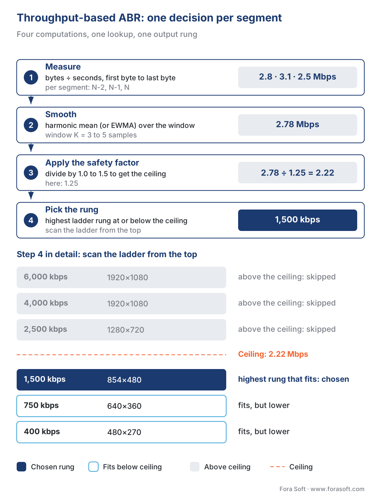 Figure 1. One decision per segment. Four computations, one lookup, one output rung.
The three production variants
Different implementations differ in which sample window they use, which smoothing function they apply, and how they handle the bootstrap. Three variants account for most of the production traffic in 2026.
Variant 1 — Plain rate-based (hls.js default)
The simplest variant. The player keeps the most recent K segments — typically 4 or 5 — in a sliding window, computes the harmonic mean, divides by a safety factor of 1.0 (yes, 1.0 in hls.js by default), and picks the rung. The hls.js team chose the lower safety factor on the grounds that the harmonic mean already biases toward conservative estimates; piling more conservatism on top under-uses the network. The hls.js source file src/utils/ewma-bandwidth-estimator.ts shows the actual implementation, which combines the per-segment throughput with an exponentially weighted moving average — abbreviated EWMA — to give more weight to recent samples within the window.
EWMA works like this: each new sample updates the estimate as new = α × sample + (1 − α) × old, where α between 0 and 1 controls how fast the estimate forgets old samples. With α = 0.5, the estimate halves the weight of every prior sample at each step. With α = 0.1, the estimate barely moves on any single sample. hls.js uses two EWMA estimators in parallel — a fast one and a slow one — and uses the lower of the two when deciding whether to drop, the higher when deciding whether to climb.
Variant 2 — ELASTIC
Published in 2014 by De Cicco, Caldaralo, Palmisano, and Mascolo as ELASTIC: A Client-Side Controller for Dynamic Adaptive Streaming over HTTP, the variant adds a PID controller — a feedback loop borrowed from control engineering — on top of the rate estimate. Instead of choosing a rung in a single divide-and-lookup step, ELASTIC defines a target buffer level and feeds the error between current and target buffer into the controller, which adjusts the effective ceiling smoothly. The advantage over plain rate-based is stability: when the network oscillates around a value that sits between two rungs, ELASTIC stays on the lower rung rather than flipping every segment. The disadvantage is the new tuning surface — PID controllers need their gain coefficients picked carefully, and bad values produce slow, sluggish reactions to real network drops.
ELASTIC ships in research code and a few commercial products; it is the conceptual ancestor of every "smoothed throughput estimator with hysteresis" you see in modern players.
Variant 3 — PANDA
Published in 2014 by Li, Begen, Erfanian, and Houdaille as PANDA: Probe and Adapt for HTTP Video Streaming, PANDA was designed to address a specific failure of plain rate-based ABR: when multiple players share a bottleneck link, plain rate-based estimators converge on a state where each player thinks it has more bandwidth than it actually does, because the measurement is contaminated by the OFF time between segments. PANDA introduces a probing rate that is updated by a control law independent of the raw segment throughput, and uses the probing rate (not the throughput) as the basis for the rung pick. The result is more graceful behaviour when ten viewers share a router uplink.
PANDA is the algorithm of record in academic comparisons and ships inside several commercial CDN-side ABR helpers. It does not ship as a default in any of the major open-source players, but the lesson it teaches — that "measured throughput between segments" is not the same as "available throughput when downloading a segment" — is now baked into every serious modern estimator.
A worked example with numbers
Set up: a 30-minute video, six-rung ladder (400, 750, 1500, 2500, 4000, 6000 kbps), 4-second segments, a viewer on a stable 3.2 Mbps DSL line.
After the first three segments, the player has measured throughputs of 3.4, 2.9, and 3.0 Mbps (TCP slow-start inflated segment 1; segments 2 and 3 are closer to steady state). The harmonic mean is 3 ÷ (1/3.4 + 1/2.9 + 1/3.0) ≈ 3.09 Mbps. With a safety factor of 1.25, the ceiling is 2.47 Mbps. The highest rung at or below 2,470 kbps is 1,500 kbps — note this is well below the actual line rate, because the safety factor is doing what it was designed to do.
The player downloads segment 4 at 1,500 kbps. The 4-second segment is 750 KB, which arrives in 1.9 seconds on the 3.2 Mbps line. The buffer grows by (4 − 1.9) = 2.1 seconds. The measured throughput for this segment is roughly 3.16 Mbps, which is close to the prior window. The harmonic mean updates marginally; the ceiling moves marginally; the algorithm picks 1,500 kbps again.
This is the algorithm's happy place. On a stable network, the rung does not change. The user sees consistent quality for as long as the network stays steady.
Now introduce a 10-second dip to 1.4 Mbps starting at second 20. Segment 6 (downloaded during the dip) measures 1.4 Mbps. The new harmonic mean is 3 ÷ (1/3.0 + 1/3.16 + 1/1.4) ≈ 2.06 Mbps. Ceiling = 1.65 Mbps. Highest rung at or below = 1,500 kbps. The algorithm stays put — the harmonic mean's protection means a single bad sample does not flip the rung.
But if the dip lasts long enough that two consecutive segments come in at 1.4 Mbps, the harmonic mean drops to 3 ÷ (1/3.0 + 1/1.4 + 1/1.4) ≈ 1.71 Mbps. Ceiling = 1.37 Mbps. The highest rung at or below 1,370 kbps is 750 kbps. The player drops one rung.
When the network recovers, the reverse happens. After three consecutive segments at 3.2 Mbps, the harmonic mean is back at 2.5+ Mbps, and the player climbs back to 1,500 kbps.
That symmetry — drop fast on sustained bad samples, climb slowly on sustained good ones — is the whole behavioural signature of throughput-based ABR. Buffer-based and hybrid algorithms make different trade-offs; throughput-based is the cleanest expression of "match the network as measured".
When throughput-based ABR is the right choice
Three deployment shapes match throughput-based ABR's strengths and forgive its weaknesses.
Shape 1 — Stable, predictable networks. Office Wi-Fi, residential fibre, satellite, and most wired connections deliver throughput that varies on the second-to-minute scale, not the millisecond scale. Throughput-based ABR's window-and-average approach fits this exactly. It picks the right rung within two or three segments and stays there.
Shape 2 — Short content. A 30-second product video does not benefit from a buffer-based algorithm's patience. By the time a buffer-based algorithm has climbed to its peak rung, the video is over. Throughput-based ABR's faster ramp-up wins here.
Shape 3 — Resource-constrained players. Embedded set-top boxes, older smart TVs, and IoT camera viewers ship with limited memory and CPU. A throughput-based algorithm needs to remember the last 4–5 samples and do one division per segment. A buffer-based algorithm tracks a continuous buffer model and a utility function; a hybrid algorithm runs both. On a 100 MHz CPU with 2 MB of RAM, throughput-based ABR is the only one that fits.
The Bitmovin Video Developer Report 2024 still found that roughly 40% of surveyed streaming engineers ship throughput-based as their primary algorithm, with buffer-based and hybrid splitting the remainder. The number has been declining year over year as Shaka Player and dash.js take more share, but it has not collapsed — for good reasons.
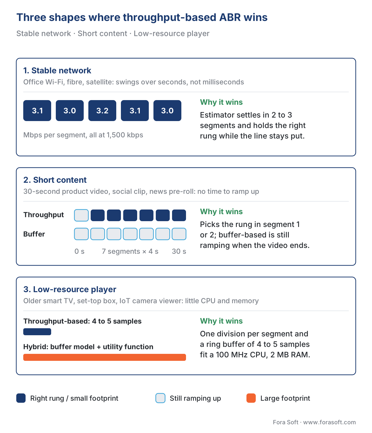 Figure 2. Three deployment shapes where throughput-based ABR genuinely outperforms more sophisticated algorithms.
Where throughput-based ABR breaks
Five failure modes account for almost every production complaint about throughput-based players. Each has a fix.
Failure 1 — Bursty Wi-Fi networks. Home Wi-Fi throughput swings by a factor of 5–10 second to second when other devices are active. A pure rate-based estimator follows the swings and oscillates the rung. The user sees the picture shift between 720p and 1080p every 8 seconds. Fix: increase the EWMA α toward 0.1 (slower forgetting), or move to a buffer-based algorithm for known-bursty environments.
Failure 2 — Mobile network handoffs. When a phone hands off from Wi-Fi to LTE or LTE to 5G, throughput jumps by 5× or drops by 5× in a single segment. The harmonic mean does not see it for two or three segments. By the time the algorithm drops, the buffer has already drained. Fix: pair the estimator with a hard floor (drop to the bottom rung immediately if buffer < 2 seconds) and a slow climb path back up after recovery.
Failure 3 — CMAF chunked transfer encoding. When the encoder uses Common Media Application Format, abbreviated CMAF (ISO/IEC 23000-19), with chunked transfer, partial segments arrive at the player as soon as the encoder produces them — at exactly the bitrate of the rung, not at the network's available throughput. A naive estimator divides bytes by seconds and concludes the network is exactly as fast as the current rung. The result: the player never climbs, even on a 1 Gbps line. Fix: measure throughput only on the inter-chunk gap (when the network was idle) or read the HTTP downloader's idle-time metric. This is one of the harder bugs in low-latency player engineering, and it shows up in production a lot. The LL-HLS Deep Dive and LL-DASH and CMAF Chunked articles cover the chunked-transfer arithmetic in more depth.
Failure 4 — Multiple players on one bottleneck. This is the PANDA failure. Five viewers on the same home router each see roughly 1/5 of the uplink, but each player's measurement assumes it owns the whole pipe. The cumulative request pattern is rough on the router's queue, and all five players oscillate together. Fix: use PANDA-style probing, or coordinate at the application layer (rare in practice).
Failure 5 — The first segment. With zero history, the player has to start somewhere. Picking the bottom rung looks bad in the first 5 seconds — the period that decides whether the viewer keeps watching. Picking too high a rung rebuffers immediately. Fix: persist the previous-session throughput across plays, and use a conservative middle rung if no history exists. Most modern players do both.
Tuning levers — the knobs that actually matter
If you ship a throughput-based player and need to tune it, four knobs do almost all the work.
Knob 1 — Window size K. How many recent samples the estimator considers. K = 3 reacts fast and oscillates; K = 8 is smooth but slow. Default to K = 5 for VoD, K = 3 for live.
Knob 2 — Safety factor. The divisor on the ceiling. 1.0 (no safety) is hls.js's default and works because the harmonic mean is already conservative. 1.25 is the most common "real-world" value. 1.5 is for networks you do not trust at all (international mobile, low-end satellite). Above 2.0 wastes too much bandwidth.
Knob 3 — EWMA α. Only relevant if you use exponential smoothing instead of a flat window. Lower α (e.g. 0.1) means slower forgetting and steadier estimates; higher α (e.g. 0.5) means faster forgetting and reactive estimates. A common production pattern: run two EWMAs in parallel, α = 0.1 (slow) and α = 0.5 (fast), and use the slow one for climb decisions, the fast one for drop decisions. This is what hls.js does.
Knob 4 — Drop hysteresis. Whether to require one bad sample, two consecutive, or a moving-average crossing before switching down. One sample is reactive; two is the most common; three is conservative. Pair this with the buffer-floor rule from Failure 2 above so that a sustained drop does not rebuffer.
The table below shows reasonable defaults for three common deployments.
| Deployment | K (window) | Safety factor | EWMA α (slow / fast) | Drop hysteresis |
|---|---|---|---|---|
| VoD on residential fibre | 5 | 1.25 | 0.10 / 0.50 | 2 segments |
| Live event on mixed networks | 3 | 1.4 | 0.15 / 0.50 | 1 segment |
| Mobile-first OTT app | 4 | 1.5 | 0.10 / 0.40 | 1 segment (+ buffer floor) |
Comparison with the alternatives
Throughput-based is one of four ABR families. The trade-offs in one table.
| Family | Primary signal | Strengths | Weaknesses | Where it ships |
|---|---|---|---|---|
| Throughput-based | Recent download rate | Simple, predictable, fast start | Jittery on bursty networks, blind to buffer state | hls.js, iOS native, older dash.js, most smart TVs |
| Buffer-based | Buffer depth in seconds | Smooth, robust under jitter | Slow to climb, mathematically dense | dash.js (BOLA) since 2018, Shaka Player option |
| Hybrid | Both, plus utility function | Best user QoE in production | Hard to debug, large parameter space | Netflix, YouTube, most premium streamers |
| Neural | Learned policy from training data | Best in benchmarks | Heavy to train, retrains needed, opaque | Research, two or three top streamers |
Common mistakes when shipping a throughput-based player
Pitfall 1 — Trusting segment 1. TCP slow-start inflates the first segment's measured throughput by 2–3×. Discard or downweight segment 1 before feeding it to the estimator.
Pitfall 2 — Not measuring switches. A throughput-based player can oscillate between rungs without rebuffering, which means the QoE damage hides from the rebuffer-ratio metric. Track switches per minute explicitly. Above 1 switch every 60 seconds, the algorithm is too reactive.
Pitfall 3 — Ignoring the buffer entirely. Pure throughput-based ABR will keep climbing into a rebuffer if the network drops faster than the smoothing window. A buffer-floor rule (drop hard if buffer < 2 s) is a small change with a large QoE win.
Pitfall 4 — Hard-coded ceilings. Capping the algorithm at "no higher than 4 Mbps for mobile" sounds prudent until you test on a 5G phone with a 500 Mbps line. Use the player's network-type signal to switch caps, not to enforce one.
Pitfall 5 — Not separating climb and drop logic. Climbing and dropping have asymmetric costs — climbing too fast rebuffers; dropping too slow rebuffers also; climbing too slow wastes bandwidth; dropping too fast looks bad. Use two estimators (fast for drop, slow for climb) instead of one.Free download: Throughput-Based ABR Tuning SheetOne printable page with the four tuning knobs (window size, safety factor, EWMA alpha, drop hysteresis), starting defaults for VoD, live and mobile, and the five failure modes each knob addresses.
Where Fora Soft fits in
We have shipped 239+ video products since 2005 and we have seen throughput-based ABR in almost every codebase we have inherited — usually because the product started with hls.js or the iOS native player and never revisited the decision. Most of the wins come not from replacing the algorithm but from tuning its four knobs against the actual viewer network distribution. In e-learning we keep throughput-based because the network is stable and the rebuffer cost is high; in mobile-first OTT we add the buffer-floor rule and a session-throughput memory; in telemedicine we move to hybrid because clinical screens cannot tolerate a quality dip during a diagnostic question. The right algorithm depends on the audience, not on what is currently fashionable in conference talks. When a team wants that tuning done on its own player, our video streaming software development work covers the ABR logic, the HLS/DASH ladder and the QoE telemetry, and for subscription services the OTT and Internet TV platform team ships it across web, mobile and Smart TV players.
The book
Video Streaming: A Complete Guide to Video Delivery: From ABR and CDNs to Players, WebRTC, DRM, and the Economics of Streaming
This article covers one ABR family. Book 3 puts it next to the others: throughput, buffer-based BOLA, hybrid MPC and neural ABR on the same ladder and the same network traces, then follows the decision into hls.js, dash.js and Shaka Player, and into the QoE metrics that tell you whether your tuning worked. Written by Nikolay Sapunov, CEO at Fora Soft.
Is your player switching rungs more than once a minute?
Send us your ladder, your player and a week of QoE data. We will check the window size, safety factor, EWMA settings and drop hysteresis against your real viewer networks, and tell you whether tuning is enough or it is time for buffer-based or hybrid ABR. 250+ video products shipped since 2005.
See our case studies
Case study
Scholarly
Test-prep e-learning for 15,000+ students, with live classes of up to 2,000 at once and adaptive DASH/HLS playback for recorded lessons.
Case study
V.A.L.T
Video recording and review for medical training and law enforcement: HLS playback on web, iOS and Android, grown from $1M to $8M in revenue in five years.
Case study
Worldcast Live
HD concerts for 10,000 simultaneous viewers at 0.4–0.5 s latency, with quality that adjusts on the fly for viewers on poor connections.
What to read next
ABR
Adaptive Bitrate Streaming Explained Without Buzzwords
The four ABR families side by side, and where throughput-based fits.
ABR
Hybrid ABR: MPC, Festive, CS2P, the Real-World Defaults
What premium streamers run when throughput alone is not enough.
Players
hls.js in Depth
The dual-EWMA estimator from this article, inside the real player.
QoE
Player Observability and the Metrics That Ship in Production
Switches per minute, rebuffer ratio: how to know your tuning works.
References
- IETF RFC 8216 — HTTP Live Streaming (Pantos and May, May 2017). Defines the multi-variant playlist that the ABR algorithm reads. §4.3.4.2 covers the variant streams. https://www.rfc-editor.org/rfc/rfc8216
- ISO/IEC 23009-1:2022 — Information technology — Dynamic adaptive streaming over HTTP (DASH) — Part 1: Media presentation description and segment formats. Fifth edition. The controlling document for DASH and the manifest format the player parses.
- Apple — HTTP Live Streaming (HLS) Authoring Specification for Apple Devices, revision 2025-09. §4.7.5 specifies recommended behaviour for initial rung selection — the algorithm's bootstrap problem in normative form. https://developer.apple.com/documentation/http-live-streaming/hls-authoring-specification-for-apple-devices
- ISO/IEC 23000-19:2024 — Information technology — Multimedia application format (MPEG-A) — Part 19: Common media application format (CMAF) for segmented media. Fourth edition. The CMAF chunked-transfer behaviour that breaks naive throughput estimators is defined here.
- L. De Cicco, V. Caldaralo, V. Palmisano, S. Mascolo — ELASTIC: A Client-Side Controller for Dynamic Adaptive Streaming over HTTP, Packet Video Workshop 2013. The PID-controller variant of throughput-based ABR. https://ieeexplore.ieee.org/document/6618416
- Z. Li, X. Zhu, J. Gahm, R. Pan, H. Hu, A. Begen, D. Oran — Probe and Adapt: Rate Adaptation for HTTP Video Streaming at Scale (PANDA), IEEE Journal on Selected Areas in Communications, 2014. The probing-rate variant that addresses bottleneck contention. https://ieeexplore.ieee.org/document/6855378
- hls.js —
src/utils/ewma-bandwidth-estimator.tssource. Reference implementation of dual-EWMA throughput estimation. https://github.com/video-dev/hls.js - DASH Industry Forum — DASH-IF Implementation Guidelines: Restricted Timing Model (v5.x, 2024). The DASH-IF profile that clarifies ISO/IEC 23009-1's ambiguities on player adaptation. https://dashif.org/guidelines
- K. Spiteri, R. Urgaonkar, R. K. Sitaraman — BOLA: Near-Optimal Bitrate Adaptation for Online Videos, IEEE INFOCOM 2016. Provides the formal contrast against which throughput-based algorithms are usually benchmarked. https://arxiv.org/abs/1601.06748
- Bitmovin — Video Developer Report 2024. Survey data on algorithm-family deployment share. https://bitmovin.com/video-developer-report
- Conviva — State of Streaming Q4 2024. Industry benchmarks for rebuffer ratio and start-up time that throughput-based algorithms drive directly. https://www.conviva.com/state-of-streaming
